GDAs with a Minimum Price
Edited on May 22, 2024 to add a missing term (\(r\)) in the price equation, which filters through the other results.
Gradual Dutch Auctions (GDAs), popularized by Paradigm, are a multiunit auction format that have some nice properties conducive to running on a blockchain. Paradigm's original definition focused on a single variable auction in which the price of the individual items was auctioned independently on a set issuance schedule. They primarily applied this to NFT mints, culminating in Variable Rate Gradual Dutch Auctions (VRGDAs) being used to control the mint speed and price for NFTs in the Art Gobblers project. However, they also defined a Continuous GDA variant for auctioning off fungible tokens (e.g. ERC20s). In the continuous case, the auction capacity is split up into infinitesimally many auctions which begin one after another over the course of the defined duration. The price of a given auction decays over time, as is customary in a Dutch Auction, at a configured speed and along a configured curve. The price is denoted as a number of quote tokens (i.e. tokens to be received) per payout token. In the reference definition, Paradigm both linear and exponential decay versions with a linear issuance schedule.
In this post, I will expand on the Continuous GDA model to introduce a non-zero minimum price for the auction. This is useful for assets where a reserve price is desired to prevent the auction from decaying below a certain value. I will focus on the exponential decay case. It can be extended to the case of linear decay, but the solutions are more cumbersome. I will use slightly different notation from Paradigm to not confuse variable names with "quote" and "payout" amounts.
Exponential Decay
Here is a quick recap of Paradigm's Continuous GDA with exponential decay, as detailed in the paper. The price in quote tokens of an individual auction with exponential decay is defined as:
$$q(t) = q_0 r e^{- \lambda t}$$
where \(q\) is the price of the auction in quote tokens, \(q_0\) is the starting price of each auction, \(r\) is the emissions rate (number of tokens sold per auction) and \(\lambda\) is the decay speed constant. The Paradigm paper does not include the emissions rate term in this equation since the idea of an infinitesimal auction can account for a single token. However, in practice, there is a discrete timestep that must be used in an implementation, e.g. a second. Therefore, we need to account for the number of tokens being sold in each auction to get its correct price.
If a user wants to purchase a quantity, i.e. payout, \(p\) of tokens from the GDA at time \(t\), they must purchase the auctions that started from \(t - T\) to \(t - T + \frac{p}{r}\) where \(T\) is the age of the oldest available auction and \(r\) is the emission rate of the auction (quantity over duration). Therefore, the current total price for quantity \(p\) would be:
$$Q(p) = \int_{T - \frac{p}{r}}^{T } q_0 r e^{-\lambda t} dt = \frac{q_0 r}{\lambda} \frac{e^{\frac{\lambda p}{r}} - 1}{e^{\lambda T}}$$
To implement an auction on this price curve, it is also helpful to be able to calculate the payout a user would receive from providing a certain number of quote tokens. We can do this by taking the inverse of \(Q(p)\):
$$Q^{-1}(p) = P(q) = \frac{r}{\lambda} \ln{\left(\frac{\lambda e^{\lambda T}}{q_0 r} q + 1\right)}$$
A nice property of using exponential decay is that we get a simple, closed-form solution to this equation.
Setting a Minimum Price
In the standard GDA model, the price of an auction always decays from the starting price to zero. This implies a certain shape to the price curve which is traversed based on the decay speed. However, we may want to set a minimum price for the auction to prevent it from decaying past a certain point. For assets with competitive markets, this likely isn't necessary, but it is a useful feature for long-tail, illiquid assets. Let's update our curve to include a minimum price \(q_m <= q_0\).
$$q(t) = r \left((q_0 - q_m) e^{-\lambda t} + q_m \right)$$
This curve decays exponentially, but only from \(q_0\) to \(q_m\). We can verify this by checking the boundary conditions:
$$ q(0) = r \left((q_0 - q_m) + q_m \right) = q_0 r $$
$$ \lim_{t \to \infty} q(t) = \lim_{t \to \infty} \left[r \left((q_0 - q_m) e^{-\lambda t} + q_m \right)\right] = q_m r $$
We can calculate the total price for a quantity \(p\) of tokens in the same way as before:
$$Q(p) = \int_{T - \frac{p}{r}}^{T } r \left((q_0 - q_m) e^{-\lambda t} + q_m \right) dt $$ $$Q(p) = \frac{r (q_0 - q_m)}{\lambda} \frac{e^{\frac{\lambda p}{r}} - 1}{e^{\lambda T}} + q_m p$$
This seemingly works, but the inverse of this function, which calculates the payout for an amount of quote tokens, is more complicated.
$$ P(q) = \frac{r}{\lambda} \left(\frac{\lambda q}{q_m r} + C - W(C e^{\frac{\lambda q}{q_m r} + C})\right) $$
where \(C = \frac{q_0 - q_m}{q_m e^{\lambda T}} \) and \(W\) is the Lambert W-function. This is closed-form, but the W-function is not commonly available, especially in smart contracts. However, we can do a reasonable job with an approximation.
A separate option would be to use the basic exponential decay curve and truncate it at the minimum price. This would be a simpler solution, but would not have the same properties as the curve we defined. We can see the difference in the following chart where both curves have the same decay factor.
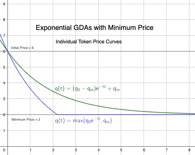
While you can achieve a similar curve with both versions by varying the decay factor. This creates a more complicated relationship between the decay speed and the minimum price, which is somewhat undesirable to make it user friendly. Therefore, let's see how we can implement the Lambert W-function in Solidity to use the preferred solution.
Lambert W-function
The Lambert W-function, also called the ProductLog function, is the inverse function of the transcendental equation \(f(x) = x e^x\), i.e. \(W(f(x)) = x\).. It appears in various solutions to exponential equations, such described here. It is, however, a complex function with multiple branches. Two of the branches are real-valued with the principal branch, denoted as \(W_0\), being defined from \((\frac{-1}{e}, \infty)\). For our purposes, I will only focus on this branch of the function from \([0, 2^{256} - 1]\) and will refer to it simply as \(W\)since we will be using 256-bit unsigned integers in our implementation. Additionally, \(W_0\) is monotonically increasing for all values in the target range, \(W_0(0) = 0\), and \(W_0(x) < x\) for all \(x > 0\). Therefore, the range of \(W_0\) will fit within our target range for the given domain.
Approximation
Since the W-function appears in various physics domains, much work has been done developing approximations for it's different branches. In 2017, Iacono and Boyd provided an overview of previous approximation methodologies and proposes a simple iterative method for approximating our target branch for \(x > 0\). We will use their method for our implementation since it has nice properties for implementation in a smart contract:
- It is defined on the exact domain we are targeting.
- The only non-native operation required is the natural logarithm, which has been implemented in multiple fixed-point math libraries to a decently high degree of precision.
- The method is iterative and converges quickly. The paper claims three iterations to a machine precision of \(10^{-16}\). We will use four iterations to get a few extra decimal places, but this can be reduced to three to save gas costs.
- It doesn't require direct multiplication of the input, which can cause overflows with large numbers.
The first step is to calculate the initial guess for the result: $$ W(x)_0 = \ln \left(1 + \frac{x}{1 + 0.5 \ln(1 + x)}\right) $$
Then, we iteratively refine the result until we reach the desired precision: $$ W(x)_{n+1} = \frac{W(x)_n}{W(x)_n + 1} \left(1 + \ln \left(\frac{x}{W(x)_n}\right)\right) $$
Solidity Implementation
For the implementation, I will use the well-tested and efficient PRBMath fixed-point math library. The library supports unsigned fixed-point numbers with 18 decimals of precision, UD60x18. It also has a decently cheap implementation of the natural logarithm, ln, which we will rely on heavily.
With four iterations, we will call the ln function six times. At an average cost of 4000 gas per call, this will cost around 24,000 gas plus the other operations. This is a reasonable cost for a complex function like the Lambert W function, though we can probably reduce it to three iterations to save gas and still get a good approximation.
Additionally, we must restrict the domain to MAX_UD60x18 - UNIT to prevent overflow when adding UNIT to the input.
import {UD60x18, ln, HALF_UNIT, UNIT, ZERO}
    from "prb-math/src/UD60x18.sol";
// UNIT is 1e18 -> 1 in fixed point
// HALF_UNIT is 0.5e18 -> 0.5 in fixed point

function productLn(UD60x18 x) pure returns (UD60x18 w) {
 // If x is zero, the result is zero.
    if (x == ZERO) return ZERO;

    // The approximation requires that UNIT
    // can be added to x without overflowing
    if (x > MAX_UD60x18 - UNIT) revert "input too large";

    // Initial guess
    w = ln(UNIT + x / (UNIT + HALF_UNIT * ln(UNIT + x)));

    // Iterative approximation
    // Four iterations gets us close
    // to 18 decimals of precision
    for (uint256 i = 0; i < 4; i++) {
        w = w / (w + UNIT) * (UNIT + ln(x / w));
    }
}
Realized Error
Initial testing of the implementation reveals pretty good results. The approximation seems to slightly underestimate the value reported by WolframAlpha. This deviation increases slightly as x increases; however, it is only 86 wei at the maximum input value of MAX_UD60x18 - UNIT = 2**256 - 1 - 1e18. The below table provides more results.
| x | WolframAlpha | Approximation | Error |
|---|---|---|---|
| \(0.1\) | 0.091276527160862264 | 0.091276527160862263 | 1 wei |
| \(0.5\) | 0.351733711249195826 | 0.351733711249195823 | 3 wei |
| \(1\) | 0.567143290409783872 | 0.567143290409783868 | 4 wei |
| \(2\) | 0.852605502013725491 | 0.852605502013725487 | 4 wei |
| \(e\) | 1 | 0.999999999999999994 | 6 wei |
| \(\pi\) | 1.073658194796149172 | 1.073658194796149166 | 6 wei |
| \(4\) | 1.202167873197042939 | 1.202167873197042932 | 7 wei |
| \(8\) | 1.605811996320177596 | 1.605811996320177591 | 5 wei |
| \(10^6\) | 11.383358086140052622 | 11.383358086140052608 | 14 wei |
| \(10^{18}\) | 37.813856075588763228 | 37.813856075588763202 | 26 wei |
| \(2^{256} - 1 - 10^{18}\) | 131.123010654220946391 | 131.123010654220946305 | 86 wei |
Appendix: Formula Derivations
Price of \(p\) payout tokens at time \(t\): $$ \begin{aligned} Q(p) &= \int_{T - \frac{p}{r}}^{T } r \left((q_0 - q_m) e^{-\lambda t} + q_m \right) dt \\ &= r \left[ - \frac{(q_0 - q_m)}{\lambda} e^{-\lambda t} + q_m t \right] \Big|_{T - \frac{p}{r}}^{T} \\ &= r \left(- \frac{q_0 -q_m}{\lambda} (e^{-\lambda T} - e^{-\lambda (T - \frac{p}{r})}) + q_m (T - (T - \frac{p}{r})) \right) \\ &= r \left(- \frac{q_0 - q_m}{\lambda} \left(\frac{1 - e^{\frac{\lambda p}{r}}}{e^{\lambda T}}\right) + q_m (T - T + \frac{p}{r}) \right) \\ &= r \left(\frac{q_0 - q_m}{\lambda} \frac{e^{\frac{\lambda p}{r}} - 1}{e^{\lambda T}} + \frac{q_m p}{r} \right) \\ &= \frac{r (q_0 - q_m)}{\lambda} \frac{e^{\frac{\lambda p}{r}} - 1}{e^{\lambda T}} + q_m p \\ \end{aligned} $$
Payout for \(q\) quote tokens at time \(t\) (inverse of Q(p)): $$ \begin{aligned} q &= \frac{r (q_0 - q_m)}{\lambda} \frac{e^{\frac{\lambda p}{r}} - 1}{e^{\lambda T}} + q_m p \\ \frac{\lambda e^{\lambda T}}{r (q_0 - q_m)} (q - \frac{q_m p}{r}) &= e^{\frac{\lambda p}{r}} - 1 \\ \frac{q_m e^{\lambda T}}{q_0 - q_m} (\frac{\lambda q}{q_m r} - \frac{\lambda p}{r}) + 1 &= e^{\frac{\lambda p}{r}} \\ \left(\frac{q_m e^{\lambda T}}{q_0 - q_m} (\frac{\lambda q}{q_m r} - \frac{\lambda p}{r}) + 1 \right) e^{\frac{- \lambda p}{r}} &= 1 \\ \left(\frac{\lambda q}{q_m r} - \frac{\lambda p}{r} + \frac{q_0 - q_m}{q_m e^{\lambda T}} \right) e^{\frac{- \lambda p}{r}} &= \frac{q_0 - q_m}{q_m e^{\lambda T}} \\ \left(\frac{\lambda q}{q_m r} - \frac{\lambda p}{r} + C \right) e^{\frac{\lambda q}{q_m r} - \frac{\lambda p}{r} + C} &= C e^{\frac{\lambda q}{q_m r} + C} \\ \frac{\lambda q}{q_m r} - \frac{\lambda p}{r} + C &= W(C e^{\frac{\lambda q}{q_m r} + C}) \\ \frac{\lambda p}{r} &= \frac{\lambda q}{q_m r} + C - W(C e^{\frac{\lambda q}{q_m r} + C}) \\ P(q) &= \frac{r}{\lambda} \left(\frac{\lambda q}{q_m r} + C - W(C e^{\frac{\lambda q}{q_m r} + C})\right) \\ \end{aligned} $$
where \(C = \frac{q_0 - q_m}{q_m e^{\lambda T}} \) and \(W\) is the Lambert W-function.